
Knowledge-Graph-First (KGF) Design
Stop overloading your contexts!


I recently wrote about taxonomies and possible representations. In this post, I’d like to explore another area - how one can make taxonomies (and knowledge graphs in general) more friendly for LLMs. This comes in response to a problem I’ve been working through: SHACL files are generally concise, making them well-suited for describing the structure of generated content. Taxonomies, however, can be far more extensive, which can create problems when handling AI token costs in LangChain contexts.
What Happens Inside LangChain and RAG
It’s worth taking a moment to talk about what exactly LangChain (and RAG) does … and doesn’t do. You can think of LangChain as the part of an LLM that manages the context. The context serves as a buffer. When you send a prompt to an LLM, LangChain loads its guardrails (instructions that both tell the LLM what to work on and, in theory, set limits on what’s allowed in the context). After this, content sources are appended to this context (including secondary “persistent” user memory and, finally, the prompt sent by the user).
Once this is all secured, the prompt is fed into the LLM's latent space, and what emerges on the other side are the result tokens from latent-space operations, like a happy-go-lucky pachinko machine. This output is frequently passed back through the context, providing historical details for what occurred.
There are problems with this architecture. The first is that the context is finite, and often comparatively small; 1 million tokens is the upper limit in many cases (Anthropic’s Opus 4.5 model has this limit). This is about the size of 6-8 contemporary novels. This may seem like a lot, but even with encodings, a large knowledge graph can easily exceed that amount, and that’s assuming it takes up everything. The structural ontology can usually fit just fine, but once you factor in taxonomies, things can get a little more dicey.
Taxonomies and Models
In my previous post on taxonomies, I discussed data molecules. Since then, it’s occurred to me that there are effectively five different types of molecules: entities, components, connectors, classifiers and schemes.
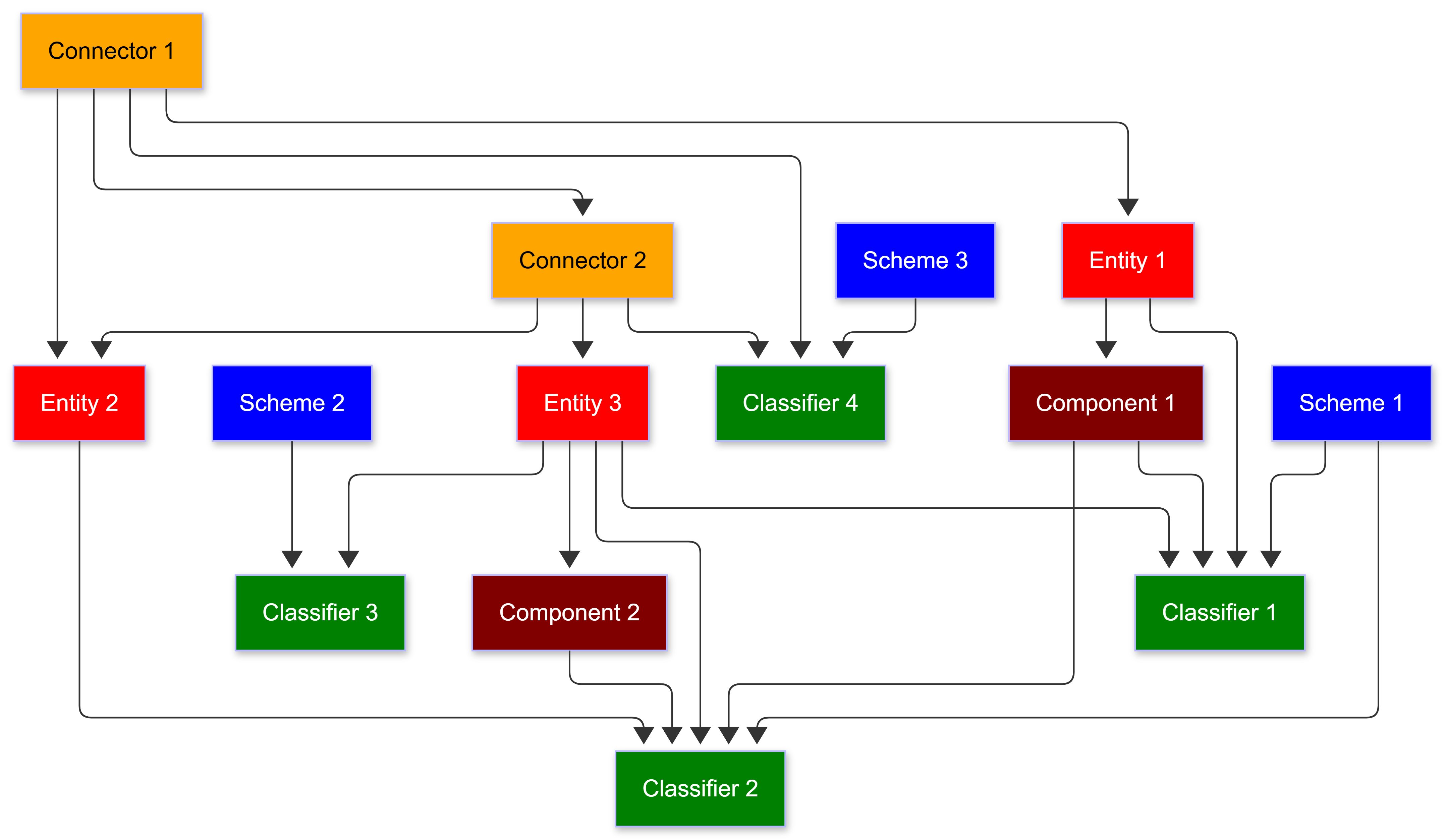
Each of these plays a different role in a given ontology.
Entities (red) typically represent physical things. They have a distinct beginning and ending, and most significantly (from a top-down methodology), they usually have very few inbound properties - they are the actors and agents in the system.
Connectors (orange) often bind multiple entities together into a contractual agreement or event. They tend to form the backbone of the ontology because they represent interactions, and as such, one interaction may connect to another to form a causal chain. A marriage, for instance, is a connector, as it is the binding between two individuals. Connectors either directly or indirectly create transitive closures.
Components (maroon) specify subordinate, more abstract entities, such as addresses (places). They are often used for composite entities, and usually have an even mix of inbound and outbound property vectors. Components are almost invariably lists in a temporal graph (a person may have multiple addresses over time).
Classifiers (Green) qualify various kinds of entities - what type of person or address, for instance - and can be applied equally to entities, connectors, and components. They are frequently the values of facets. Classifiers typically have many input vectors and relatively few output vectors, and in data models they are often represented as enumerations and may have an implicit order. They are members of various schemes.
Schemes (Blue) are sets of classifiers, each of which is a member of the set. A facet is a property of an entity whose object is a member of a scheme. For instance, if you have a scheme of colours, then the facet is ex:hasColor, and the facet value is the classifier ex:Green or ex:Purple. Schemas typically have only outbound links.
This isn’t complete; there are a few other kinds of resources that I’m not covering here, but it provides enough for making the argument.
You can argue here that this is a form of upper ontology. I’ve always been a little sceptical of the notion of upper ontologies, in part because they frequently become the basis for religious wars, but yes, from the standpoint of OWL, this is part of an upper ontology.
In most ontologies, there is usually one preferred or primary facet, typically designated by rdf:type. There is nothing magical about rdf:type - you could just as readily say ex:hasPrimaryClassOf , but every classifier that an entity has partitions the entity in a particular set. Thus, I can say
ex:JaneDoe rdf:type ex:Person .or
ex:JaneDoe rdf:type ex:Female .or
ex:JaneDoe rdf:type ex:Teacher .and each of these are true. In SHACL, you could in fact identify each of these as properties and then expose additional properties based upon what rdf:type is, but we usually tend to associate a dominant type to entities to determine how the system usually treats them.
Both entities and classifiers are members of a set, but the distinction is that entities typically have properties derived from rdf:type while classifiers derive from rdf:member. Put another way, entities are Things, classifiers are Concepts.
Where this gets problematic is in determining what constitutes a class of instances vs a scheme of concepts. For instance, is a country a thing or a concept? Is a state? How about a person or a store? This is where OWL can get very complex, because obviously, each of these could be both.
I tend to adopt a pragmatic view and consider the knowledge graph. In general, the physical things that you are concerned about, the ones that have relatively few inbound links but lots of outbound links, work best as entities in the system. Those things (usually more abstract and conceptual) that qualify entities in some way or are effectively the classifiers in the system. In most knowledge graphs, for instance, both states and countries will typically be referred to by addresses of some sort - unless it is a geopolitical knowledge graph, and in that role they are classifiers. In that case, both the country and the state will be entities. As an ontologist, one of your roles is to determine the priority of any given concept in the system to establish that distinction.
Searching Resources by Metalabels
One reason for making this distinction is that sets of facets are frequently used to select entities, because entities are composed of facets and facet values (classifiers). This means that if you can specify enough of these facets, then you can retrieve a list of entity candidates that have those facets. For instance, if I say that I’m looking for all brunette women who live in Washington and are teachers, then I have five facets (species, hair colour, gender, location, profession) that can then be used to narrow down the total population significantly through set intersection.
There are two specific use cases to consider: when the number of potential classifiers is relatively low, it is reasonable to use enumerated classes as facet values. For instance, there are probably only about a dozen hair colours unless you’re building an application for a hair products company. On the other hand, if you have hundreds or thousands of potential values in the enumeration, then you may be better off working with literal values.
This trade-off is one that many ontologists wrestle with; part of this stems from search. A literal is (in most cases) a leaf in a graph - there are one or more directed edges that point to it, but literals by their very nature usually shouldn’t have any outbound edges (there are exceptions to this, but they are rare).
Literals are strings more than they are concepts. Matching a concept is trivial - you have an existing IRI. Matching a string requires taking into account case, stemming, spelling variations, synonyms, acronyms and perhaps even descriptions. Most semantic search systems ultimately involve mapping several potential labelling vectors to a single IRI. For instance, the following (showing the label and description content for a Baritone Saxophone) is typical for a classifier:
ex:BaritoneSaxophone a ex:MusicalInstrument ;
     rdfs:label "baritone saxophone"@en, "Baritonsaxophon"@de,
     "saxophone baryton"@fr;
     rdfs:comment """The baritone saxophone is a member of the saxophone family of instruments, larger than the tenor saxophone, but smaller than the bass. It is the lowest-pitched saxophone in common use — the bass, contrabass and subcontrabass saxophones are relatively uncommon. Like all saxophones, it is a single-reed instrument.""" ;
     ex:altLabel "bari sax","bari","baritone","sax","saxophone" ;
     ex:soundsLike "prtnsksfn","prtnsks","brsks","brtn","sks" ;
     ex:acronym "BRSAX" ;
     .
In general, the goal of such an entry is to provide as many potential matching surfaces as possible without performing any computation. The reason for this is simple - if you can create a direct literal match to a property, the classifier becomes a simple index loopup (which is VERY fast), while if you have to do a starts-with, contains() or, worst case, a regex() check, you dramatically increase the time to complete a query.
By the way, the ex:soundsLike property is one of my favorite tools for cutting down on query time. It is based upon the Double Metaphone algorithm, developed by Laurence Phillips in 2000 and works by reducing words to their simplest phonetic representation. For instance, “Baritone Saxophone” reduces to “prtnsksfn”. Note that there are a few other terms that also reduce to this (“Britain Sex Fun”, oddly enough), but, in general, this can minimise lookup time significantly while reducing the need to invoke this within a SPARQL query if it’s already prewritten into the data model.
A query to find matches can then use a list of potential “metalabels”, various kind of labels that might provide different ways of finding information.
# SPARQL
# ?q = the string to be matched.

SELECT ?s ?q WHERE {
    VALUES ?q { "baritone sax" "prtnsks" "brsax" "bari sax" }
    ?s (rdfs:label|ex:soundsLike|ex:acronym|ex:altLabel) ?q .
}
In this case, the prompt illustrates four different tokens that match a particular query term ?q in the given order (label, sounds like, etc.). The query will return both the resource subject ?s and the particular query term that matched for that resource.
Note that you can do something similar with predicates. In this particular case, we’re going to extend a predicate such as ex:playsInstrument (assuming a class of ex:Person)
ex:Person_playsInstrument a PropertyShape ;
     sh:name "plays" ;
     sh:path ex:plays ;
     ex:soundsLike "pls","plsnstrmnt","plsmsklnstrmnt ;
     ex:altLabel "plays musical instrument","plays" ;
     sh:class ex:MusicalInstrument ;
     .
This changes this a bit in the SPARQL query, but not dramatically:
# SPARQL
# ?q = the string to be matched.

SELECT ?s ?q WHERE {
    VALUES ?q { "plays" }
    {{
    ?s (rdfs:label|ex:soundsLike|ex:acronym|ex:altLabel) ?q .
    UNION {
    ?p  (rdfs:label|sh:name|ex:soundsLike|ex:acronym|ex:altLabel) ?q .
    ?s ?p ?o .
    }}
}
In this case, the query is a union of two queries: the first matches a given object with its label term or synonym, the second retrieves all triples in which the predicate has the associated metalabel.
Once you have this, then the most likely matches for the given prompt can be determined by adding a match count:
SELECT ?s (COUNT(DISTINCT ?match) AS ?matchCount) WHERE {
    VALUES ?q { "plays" }
    {
        VALUES ?directProp { rdfs:label ex:soundsLike ex:acronym ex:altLabel ex:stem }
        ?s ?directProp ?q .
        BIND(?directProp AS ?match)
    }
    UNION
    {
        VALUES ?labelProp { rdfs:label sh:name ex:soundsLike ex:acronym ex:altLabel }
        ?p ?labelProp ?q .
        ?s ?p ?o .
        BIND(?p AS ?match)
    }
}
GROUP BY ?s
ORDER BY DESC(?matchCount)
The group by groups the output by the subject, making it possible to use the COUNT(DISTINCT(?match)) aggregation in the select statement, then orders them from the largest (the subject has the largest number of matching terms) to the smallest (the subject has only one match. If there are no matches, then nothing will get returned.
I snuck the ex:stem property into the mix as well. A stem in linguistics is the most basic form of a particular word. For instance, for “plays” or “playing”, the stem is “play”. Stems can also be calculated a priori and added to the index you’re building of metalabels within the graph.
There’s one more way that you can extend the matches - take advantage of doing the same to classes that you have to labels:
ex:MusicalInstrumentShape a NodeShape ;
     sh:targetClass ex:MusicalInstrument ;
     sh:name "musical instrument" ;
     ex:pluralName "musical instruments","instruments";
     ex:altLabel "instrument"
     ex:soundsLike "msklnstrmnt","nstrmmnt" ;
     ex:property ...
     .
In this case, the query can be both extended and simplified:
From prompt, include matching predicates
SELECT ?s (COUNT(DISTINCT ?match) AS ?matchCount) WHERE {
    VALUES ?metalabel { rdfs:label ex:soundsLike ex:acronym ex:altLabel
                      sh:name ex:pluralName ex:stem }
    VALUES ?q { "lisa"|"simpson"|"plays"|"bari"|"sax"|"exceptionally"|"well"} }
  {
    # find all resources that have the appropriate metalabel
    {
        ?s ?metalabel ?q .
        BIND(?metalabel AS ?match)
    } UNION
    # find all classifiers that have the appropriate metalabel
    {
        ?s ?p ?o .
        ?o ?metalabel ?q .
        BIND(?o AS ?match)
    }
    UNION
    # find all properties that have the appropriate metalabel
    {
        ?p ?metalabel ?q .
        ?s ?p ?o .
        BIND(?p AS ?match)
    }
    UNION
    # find all classes that have the appropriate metalabel
    {
       ?s a ?class .
       ?class ?metalabel ?q .
       BIND(?class as ?match)
    }
  }
}
GROUP BY ?s
ORDER BY DESC(?matchCount)
The values clause in this case can now be seen as the query prompt decomposed into individual terms. In this case, it will find the closest matches for records that may indicate that Lisa Simpson plays the bari sax (as any fan of The Simpsons probably knows). On the other hand, a different query prompt can be made:
“Who is well known for playing the bari sax?”In this case, the operant matching terms are “playing”, “bari” and “sax”, which creates a much more open-ended query. You can also add “who” to the list of altLabels for ex:Person so that there is an association there, just as you can add “where” to ex:Place to do the same for locations, “when” to ex:Event , and so forth.
Note that such queries are likely going to be slower than if you write an explicit SPARQL query, but it still provide a good natural language mechanism to be able to retrieve resources that may match the desired prompt.
Understanding KGF Design
There is one caveat to this approach - unlike an LLM, where being verbose is likely to provide a better match (because it is comparing similarity vectors), with a semantic query, there’s a point at which more text likely will not materially change what you get back, and what you get back will be primarily a list of resource links with a thin layer of metadata. Semantic graphs generally do not readily lend themselves to similarity vectors, as they are built on different principles. However, if similar graph properties reference different text nodes, you can compare those referenced text nodes through such similarity graphs.
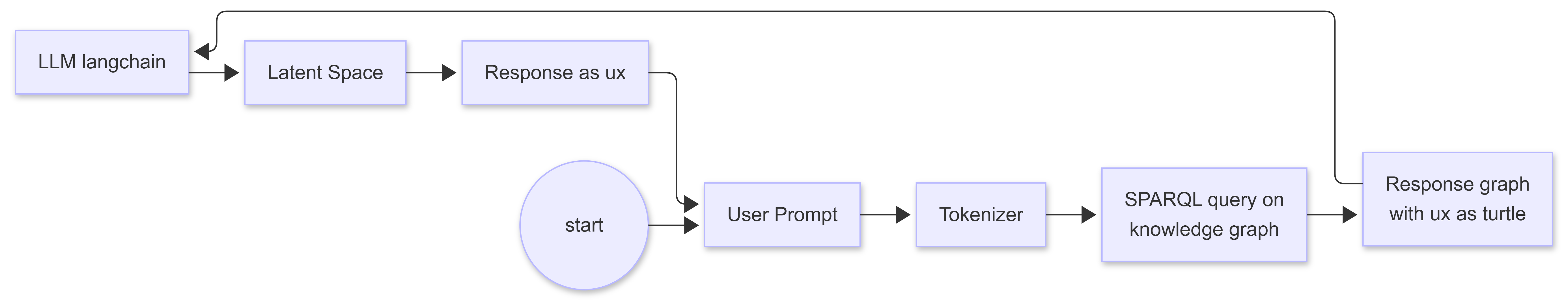
An interesting implication of this is that it suggests that prompts may be better performed by first querying a knowledge graph to get the best fitting responses (or perhaps just the first best response) as a list of nodes with metadata, then, upon determining a threshold of potential valid answers, retrieving the graphs of that node and passing those graphs to the LLM context.
The “traditional” LLM architecture with graph rag looks something like the following:
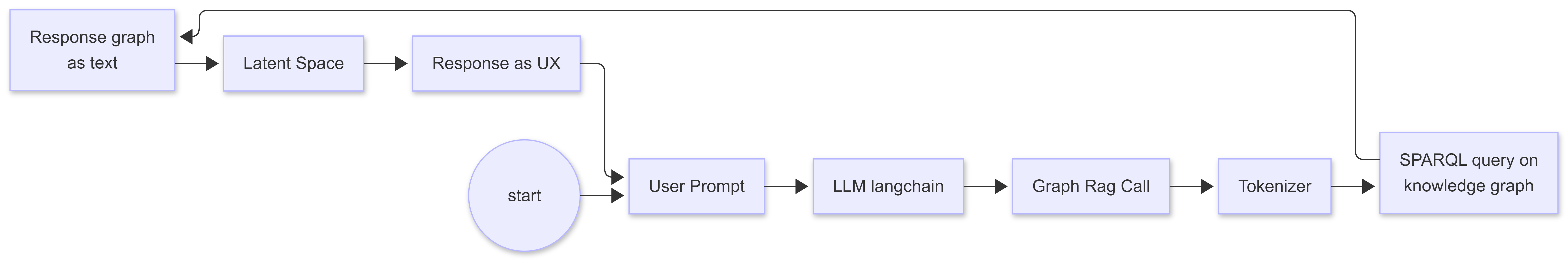
In the case of the statement “Lisa Simpson plays the bari sax”, as an example, this will retrieve the nodes that describe Lisa Simpson, playing a musical instrument, and the baritone saxophone. These, in turn, can be passed as Turtle to the prompt, along with the initial SPARQL prompt. This is Knowledge-Graph-First Design.
So, why should Turtle be passed in this manner? Would it be preferable to pass it as natural-language text or as JSON? Maybe not. Most LLMs are actually trained to work with Turtle (among other languages), and the pattern-matching capabilities inherent with LLMs are surprisingly good at manipulating the declarative, articulated structure of graphs with token IRIs - especially if those IRIs are condensed as curies (which is essentially what Turtle does).
In that respect, Turtle is a superfood to LLMs - the pattern searching and matching are already partially done when you pass Turtle to the langChain, which is part of the reason why graph-RAG type approaches generally improve both the performance and the accuracy of the resulting response.
However, there’s another reason why querying the knowledge graph first is preferable to inserting it mid-chain. Most of the queries that people write initially with LLMs are effectively searches - find these people, this location, this quotation, these products. Even when generating content, such as an image or video, these users typically form a conceptual image they seek to find in a virtual space. In effect, the graph serves as a world model, identifying those nodes that are most relevant to the prompt and using those to paint a more detailed (and consistent) picture.
This may not be desirable when you’re looking to engage in free association. However, in many cases, the goal is to provide the relevant background information to an LLM, possibly with additional schematic metadata to aid interpretation, enabling the LLM to transform the output into meaningful natural language and to augment it with further information.
This solves another problem with working with knowledge graphs. As was discussed earlier, knowledge graphs can be both large and dense, and transferring a knowledge graph into a limited context is often simply not efficacious - especially when dealing with taxonomy information that may be extensive. So don’t put that information into the context in the first place. Instead, put a structural schema into the context to help inform the model, and a graph that obeys that schema, consisting of the results of the query, that can then be passed (along with the prompt) to the LLM.
Now, this probably doesn’t sound attractive to those who see LLMs as being primary sources of information, and who feel that if you don’t have transformers driving everything, then this isn’t REAL AI. That’s so much BS. Consider, for instance, what could happen with a knowledge-graph first approach. You could define not only data structures and curated data but also create pipelines for processing that information with a comprehensive schematic understanding of the system at hand. Such a pipeline would be declarative, fully transparent, and consistent from one run to the next.
What’s more, that graph can be updated in real time - you don’t have to wait six months and spend hundreds of millions of dollars to create new training data; the data is available the moment that you log a transaction. The graph may also contain relevant user interface information. When a new prompt is created, this, in turn, drives a different set of queries that are more controllable through a graph than through an LLM, which primarily serves as the renderer of that information and the mechanism for sending the user response back to the knowledge graph.
One additional benefit of this approach is that the resources passed contain referenceable identifiers that can, in turn, be returned to the knowledge graph as additional prompts. This means that over the course of the session, the LLM doesn’t slowly “forget” which items it is working with (or their structures).
A knowledge-graph-first approach takes more work to build, but it is also far more consistent, requires far fewer tokens to perform what should be routine work, and can deal with changes in state much more rapidly than an LLM-first approach. What’s more, it’s not bound by context - the output contains the schema and just enough of the taxonomy to be able to describe the result set being passed into the LLM fully.
One additional benefit of this approach is that you can identify in the result set queries (or Dynamic SHACL, once this reaches a critical point) that represent alternatives in the LLM output, which can then be passed as part of the succeeding incoming prompts of the user. Once again, you’re shifting things back from using the LLMs as an orchestrator - something that is proving increasingly untenable - to using the knowledge graph as the orchestrator for successive, consistent, predictable actions. This reduces the potential for malicious code injection by either the user or a man-in-the-middle, since what is passed is not raw code but instead, IRI references to code that exists solely within the knowledge graph.
This change in architecture removes the LLM from serving as the system's data store, relegating it primarily to those areas where it actually does best - classification, transformation, and (arguably) presentation. It doesn’t make software press-button easy, but frankly, I think this attribute is vastly over-rated; if your software is not consistent, maintainable, and secure, then at some point you are guaranteed to have a business that is locked out because a critical system has hallucinated a function that doesn’t exist.
In Media Res,

Check out my LinkedIn newsletter, The Cagle Report.
I am also currently seeking new projects or work opportunities. If anyone is looking for a CTO or Director-level AI/Ontologist, please get in touch with me through my Calendly:
If you want to shoot the breeze or have a cup of virtual coffee, I have a Calendly account at https://calendly.com/theCagleReport. I am available for consulting and full-time work as an ontologist, AI/Knowledge Graph guru, and coffee maker. Also, for those of you whom I have promised follow-up material, it’s coming; I’ve been dealing with health issues of late.
I’ve created a Ko-fi account for voluntary contributions, either one-time or ongoing, or you can subscribe directly to The Ontologist. If you value my articles, technical pieces, or general reflections on work in the 21st century, please consider contributing to support my work and allow me to continue writing.
Very insightful, I can't seem to get enough of this, though.